ABSTRACT
Positioning technology is progressing at a rapid pace. One of the latest developments is the availability of Global Navigation Satellite System (GNSS) receivers. RTK (Real Time Kinematic) GNSS receivers have the potential to increase satellite coverage and improve satellite geometry with the additional available satellites from the GLONASS constellation. This will prove beneficial to users who work in difficult operating environments such as open pit mines or urban canyons. This research is interested in the effect of difficult operating environments (i.e. obstructed satellite window and high multipath presence) on the RTK GNSS receiver’s ability to operate.
This research project has tested and compared the performance of an RTK GNSS receiver to a RTK GPS (Global Positioning System) receiver. The antenna was setup in a difficult operating environment where there was a multipath presence, and almost half of the satellite window was blocked. An analysis of the results allowed conclusions to be made about the compatibility of the combined GNSS satellite positioning frequencies of GPS and GLONASS satellites in a difficult operating environment, and about the effectiveness of a multiple frequency GNSS to mitigate multipath compared to a receiver observing solely GPS satellites.
From the results of the tests, it was found that the GNSS receiver has a superior ability to mitigate errors associated with multipath. This was demonstrated as the GNSS receiver had 7% less outlying observations than the GPS receiver in a high multipath environment. The GNSS receiver also had 33 more initialisations and a decreased time to first fix (TTFF) of 17 seconds. The results indicated that the GNSS receiver’s accuracy and precision was comparable to the GPS receiver.
This research shows that users who work in difficult operating environment (i.e. obstructed satellite window, high multipath) will benefit from the advantages of an RTK GNSS receiver which include; increased satellite coverage, improved TTFF and increased initialisation reliability.
Limitations of Use
This blog is a copy of my dissertation completed in 2007. Persons using all or any part of this material do so at their own risk.
This dissertation reports an educational exercise and has no purpose or validity beyond this exercise. This document, the associated hardware, software, drawings, and other material set out in the associated appendices should not be used for any other purpose: if they are so used, it is entirely at the risk of the user.
NOMENCLATURE AND ACRONYMS
The following abbreviations have been used throughout the text:-
DOP Dilution of Precision
EU European Union
FOC Full operation capability
GLONASS Global Navigation Satellite System
GNSS Global Navigation Satellite System
GPS Global Positioning System
NMEA National Marine Electronics Association
OTF On the fly
PDOP Precision Dilution of Precision
ppm part per million
PSM Permanent Survey Mark
RMS Root Mean Square
RTK Real Time Kinematic
TSC2 Trimble Survey Controller 2
TTFF Time to First Fix
VRS Virtual Reference Station
USA United States of America
UTC Universal Time Coordinated.
CHAPTER ONE – INTRODUCTION
1.1 Background
For almost the past three decades the United States of America (USA) has been the sole provider of an operational Global Navigation Satellite System (GNSS). This is now in the process of changing. Russia is rebuilding their GNSS GLONASS and Europe will be launching a GNSS named Galileo (Defining the Future of Satellite Surveying With Trimble R-Track Technology 2006). It is also expected that China will have a GNSS called Compass. While it is expected to provide position signals across China by 2008, it is unknown when it is expected to reach full operational capability (FOC) (Thomson 2007).
All three systems (GPS, GLONASS and Galileo) will be interoperable (GNSS 2006). The combination of the three GNSSs could result in an eventual 60+ satellite constellation by year 2010. This increase in satellite availability will be an advantage in areas where satellite availability is limited, such as in open pit mines or in urban environments (Lachaleppe et al. 2002).
Real-time kinematic (RTK) Global Positioning System (GPS) positioning has revolutionised the surveying profession (Trimble 2001). This surveying technique has increased productivity in almost all of the disciplines related to surveying. The reason RTK GPS is so productive is its achievable accuracy in real time. RTK GPS is a relative positioning technique. It reduces errors that are common to both the base station and roving receiver such as ionosphere and troposphere delay allowing RTK GPS to be used for high-accuracy applications. RTK GPS relies on GPS biases being eliminated, or at least minimised at both the receivers.
Multipath is an error which occurs when the signal from the satellite does not travel the direct route to the receiver. The amount of multipath at a receiver is determined by the surrounding environment, thus it is almost impossible to have equal amount of multipath at both antennas. Mitigating errors caused by multipath is crucial to achieving high accuracies, currently there is a need for more practical testing on the effect of multipath on a GNSS receiver’s ability to initialise.
Accuracy, precision and time to first fix (TTFF) is closely correlated to the number of available satellites, the geometry of the satellites and the presence of errors due to multipath. O’Donnell et al. (2003) and Feng et al. (2006) have stated that with the availability of more satellites in the GNSS there will be a likely improvement in the satellite geometry, thus improving the accuracy, precision and TTFF of RTK GNSS under normal conditions.
Lau (2005) created a simulation of a fully operational capable (FOC) GPS and Galileo constellations and found that in the presence of multipath the positioning results degraded further than when the receiver was observing solely GPS. This result creates uncertainty about the combined use of GPS and GLONASS. Will the combined use of GPS and GLONASS satellite signals improve the receiver’s ability to provide an accurate fixed position in the presence of multipath, or will the quality of the position results be further degraded due to compatibility issues between GPS and GLONASS?
1.2 Research aim and objectives
Aim:
The aim of this research project is to critically analyse the ability of an RTK GNSS receiver to provide more accurate and precise positioning results in a low and high multipath environment compared to an RTK GPS receiver.
Objectives:
To achieve the aim the following elements will be tested and analysed:
- Number of fixed solutions;
- Time to first fix (TTFF);
- Accuracy; and
- Precision.
1.3 Justification
Currently RTK GPS users have been using positional information from GPS only. With GLONASS being replenished and an expected fully operational Galileo satellite constellation by 2010 (Lau 2005, p. 43) it is required that research be undertaken to determine what effect these additional frequencies have on the positioning ability of receivers when used in conjunction with GPS, in particular in areas where conditions are considered less than ideal. Will the additional available frequencies from GLONASS and eventually Galileo being used in conjunction with GPS provide greater satellite coverage, more accurate and precise positioning results and faster TTFF by mitigating multipath errors more effectively?
The results of this testing will be beneficial for both users of RTK GPS and RTK GNSS receivers as the performance of the two receiver configurations will be analysed in both a low and high multipath environment so the multipath mitigation capabilities of the receivers can be determined. As a result of this testing an analysis of the benefits of wider satellite coverage will also be determined by analysing and comparing the performance elements specified in section 1.2. This will result in a conclusion able to be made as to the compatibility of GPS and GLONASS in a low and high multipath environment.
This research will also be applicable to users of Virtual Reference Station (VRS) RTK. Currently the majority of VRS RTK networks use GPS information only, knowing the performance of GNSS receivers under difficult conditions (i.e. high multipath) compared to GPS receivers will assist in deciding whether it would be an appropriate investment to upgrade VRS networks to observe information from satellites other than just GPS.
1.4 Outline of research
Chapter one has identified the need to critically analyse the ability of a GNSS capable receiver to provide more accurate and precise positioning results compared to a receiver observing solely GPS in a high and low multipath environment.
A suitable test site will first have to be found to ensure the aim and objectives can be properly assessed. As it is a requirement that each of the testing period be over a 24 hour period to ensure that observation periods are comparable, having access to a mains power outlet to power the laptop and receiver is essential. The test site will also have to represent a situation which is commonly faced by spatial professionals where it may be difficult to gain a fixed solution using a GPS receiver.
Once the data has been collected using instruments and software which will be discussed in more detail in Chapter 3, a statistical analysis of the observation data using Microsoft Excel will be completed. It is from this statistical analysis that a comparison between GNSS and GPS will be able to be made, and a conclusion drawn as to the effect of the additional satellite frequencies on the receiver’s initialisation integrity.
1.5 Limitations of Study
As this project follows on from both Manuel’s (2000) and McCabe’s (2002) project of receiver testing, it is assumed the readers of this dissertation have some knowledge of the fundamentals of GPS, initialisation integrity, good and bad initialisations and ambiguity resolution. Readers with little or no knowledge of this topic will benefit by referring to GPS texts which should be available in most libraries. Another source of information is the Trimble Navigation homepage website (www.trimble.com and click on “GPS Tutorial”). This site provides instruction on the basics of how positions are determined on the earth and more detailed information about GNSS.
1.6 Summary
Multipath is a common undetectable error in RTK GPS surveying. Research will be undertaken to determine whether the use of a GNSS enabled receiver will enhance the receiver’s ability to mitigate errors caused by multipath compared to a receiver observing solely GPS satellites.
As the GNSS receiver will be observing additional satellite frequencies from GLONASS as well as GPS it is expected that the wider satellite coverage will result in an increased chance of initialisation. It is expected that the additional available satellites will improve the elements related to receiver performance, however it is difficult to determine at these early stages if the receiver performance will improve as a greater number of satellites become available. This uncertainty is a result of the research completed by Lau (2005) which found compatibility issues between the two GNSS constellations GPS and Galileo. This research is given in more detail in section 2.4.4.
In chapter two a literature review will provide the history and development of GNSS to the present, and what may be expected in the future with regards to possible development, and expansions.
CHAPTER 2 – LITERATURE REVIEW
2.1 Introduction
To achieve the aim and objectives stated in Chapter 1, a comprehensive review of all current literature will be necessary. This will establish the current understanding and knowledge with respect to GNSS and the results of past tests, and to identify previous testing procedures so these can be adopted where appropriate for the required testing of this project.
The literature review will introduce the RTK surveying style and the benefits it has provided the users of spatial information. It will also discuss the history of GNSS, and discuss any testing methodology previously used for testing RTK receivers.
This chapter includes background information about GNSS as well as detailing past testing and the results of these tests. It will also continue to explain why it is necessary that GNSS receivers be tested in a high multipath environment by identifying the current lack of research in this research topic.
2.2 Background
With the additional position signals from GPS, GLONASS and Galileo, GNSS receivers have the potential to offer users numerous benefits over those who use receivers only able to receive GPS signals. A brief history and clarification of the expected benefits of GNSS will be explained in more detail in the following sections.
2.2.1 What is GNSS?
GNSS refers collectively to all of the global navigation satellite constellations. Currently the world’s GNSS comprises the United State’s GPS, the Russian Federation’s GLONASS, the European Union’s (EU) Galileo (Defining the Future of Satellite Surveying With Trimble R-Track Technology 2006), and China’s Compass (Thomson 2007). It is expected by 2010 (when it is expected Galileo will reach full operational capability (FOC) that there will be a 60+ satellite GNSS between GPS, GLONASS and Galileo (Gibbons 2006). It is unknown when Compass will be operational, or even if it will be designed so it is compatible with the current three GNSSs in operation, it has the potential however to reach FOC before Galileo as Compass does not have the same funding issues (which China is also investing in) (Compass GPS 2007).
2.2.2 Potential benefits of GNSS
Provided GPS, GLONASS and Galileo are interoperable, there are a number of potential benefits which will result from the added available satellites. These potential benefits are:
- Accuracy: Dilution of Precision (DOP) is a measure of the effect the satellite geometry will have on accuracy. With the availability of a greater number of satellites, an improvement in satellite geometry will result, thus there will be a resultant improvement in accuracy (Wolf & Ghilani 2002, pp. 344-5).
- Increased satellite coverage: It is sometimes difficult to gain an initialisation when working in urban canyons and steep terrain due to the view to satellites being obstructed. With a greater number of satellites, instances of this problem occurring will lessen (Lachaleppe et al. 2002).
- Measurement redundancy: Higher redundancy would result in a reduction of random errors, including phase noise and multipath effects. This improvement would lead to greater repeatability of measurements (Feng, Rizos & Moody 2006, p. 11).
- Time To First Fix (TTFF): With additional satellites available, it will be possible to resolve the inter-ambiguities faster, allowing for more productive hours of work (Feng, Rizos & Moody 2006).
2.2.3 Real Time Kinematic (RTK) surveying
‘RTK surveying is a carrier phase based relative positioning technique’ (El-Rabbany 2002, p. 77). Measuring the phase of the signal as opposed to the code allows for high accuracies to be achieved. The phase signal can be read to 1/100th of a wave length (i.e. 2mm) (Higgins 2006).
High accuracies are achieved by having a base station established on a known station. The base station will be observing the same satellites as the rover station. The base station will calculate a correction to apply to the raw satellite observations so it is at the specified coordinates. This correction will then be broadcast to the roving receiver, thus enabling points to be positioned within 1 – 5 centimetres in real-time.
One of the obvious advantages of this technique is that the information is processed in real-time, so not only is there no post-processing to do, but also points can be set out with the known accuracy of each point shown on the screen of the controller. A fixed solution can also be obtained ‘on the fly’ (OTF) with just a few epochs of data (Geodetic Surveying A – Study Book 2 2005). This means less time is spent waiting for the receiver to reinitialise.
2.3 Errors in GNSS observations
The RTK GNSS system is not infallible. There are numerous influences which affect the receiver’s ability to effectively resolve the phase integer ambiguities. Several are:
- Observation time;
- Number and geometry of satellites at time of observation;
- Quality of starting coordinates;
- Broadcast vs. precise ephemeris;
- Ionosphere and troposphere delay;
- Site specific errors such as multipath and electromagnetic interference.
(Higgins & Honor 1999)
A number of these errors, such as ionosphere and troposphere delay, are already minimised in RTK GNSS. Nearly all the errors mentioned are common to both base and rover receivers over short to medium baselines (Lau 2005, p. 26), because of this centimetre to millimetre accuracies are achievable. Multipath and electromagnetic interference are errors that are generally not in common with both receivers, this has the potential to cause errors. As the focus of this project is to research the effects of multipath on receiver initialisation, this effect will be discussed further in the following section.
2.3.1 Multipath
Multipath errors are caused when direct signals from satellites are mixed with satellite signals which have not travelled directly to the receiver but have been reflected from objects in the vicinity. This effect is shown in Figure 2.3.1.
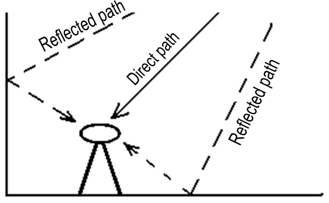
Because the receiver determines its position by resolving the number of unknown integers between itself and the satellite, a signal that travels a longer distance than is necessary will then contribute to a bad initialisation.
There are four primary influencing environments which determine the size of the multipath error: the reflecting environment; satellite geometry; the type of antenna used; and the receiver hardware used (Lau 2005, p. 51). The reflecting environment is the primary driver of this effect, the higher the reflective properties of the surface the greater the instance of the presence of multipath. The geometry of the satellites can impact on the amount of multipath. Leick (1995) believes satellites located at low elevations contribute to an increase in multipath. This is due to the low angle of elevation above the horizon, the signal is more likely to have been reflected off the ground prior to arriving at the receiver. To remove ground bounce multipath from low lying satellites, manufacturers recommend applying an satellite elevation mask so the receiver will not track these low lying satellites (Trimble SPSx80 Smart GPS Antenna – User Guide 2006, p. 120). Also antennas are now being built with internal ground planes which prevent ground bounce multipath. There has been little development in the way of receiver hardware for dynamic surveying applications which has been able to prevent multipath (Lau 2005, p. 51). Coupled with the trend towards shorter occupation time (Geodetic Surveying A – Study Book 2 2005, p. 13.1) multipath is likely to remain a serious and common error for many GNSS applications for the near-term.
2.4 Previous Receiver Testing
2.4.1 Research Undertaken by Lemmon & Gerdan (1999)
The aim of Lemmon and Gerdan’s (1999) research project was to analyse the effect of the number of satellites on the accuracy of RTK positions. The testing process was automated by using a computer program which controlled the operation of the roving GPS receiver. The primary function of this program is to extract RTK position information, which included the number of satellites and PDOP values before forcing the receiver to reinitialise (Lemmon & Gerdan 1999, p. 66). There were four separate tests completed, the time duration of each test ranging from 21 – 25 hours. The test receiver was situated ten kilometres from the base station.
Gerdan and Lemmon (1999, p. 69) concluded “that an increase in available satellites made no significant contribution to the accuracy of the RTK positions, although the reliability of the ambiguity resolution process did improve.” There was a reduction in PDOP values as more satellites became available, however when a comparison was made between the precision and accuracy of the points collected when five and nine satellites were observed the difference was negligible. This suggests that satellite geometry or the number of satellites available doesn’t impact the accuracy of RTK GPS. However, there were benefits of having a greater number of satellites available, as shown in an improvement of 75 seconds between the TTFF of a nine satellite constellation compared to a five satellite constellation (Lemmon & Gerdan 1999, p. 67).
To analyse the observations to determine the accuracy and precision of the observations, the data was required to be filtered of outlying observations. An outlying observation was considered to be more than three times the manufacturer’s specification for baseline component standard deviation. Out of the four tests completed almost 3000 points were recorded, and of these 49 or 1.7% were considered outliers. If one cluster of outlying initialisations is removed when it is expected that an obstruction was present, the resolution reliability would have exceeded 99%.
2.4.2 Research Undertaken by Manuel (2000)
Manuel (2000) completed a critical analysis of the Trimble 4700 receiver. To properly assess the receiver’s ability to initialise correctly, three different test sites were selected to test receiver performance under different operating environments. One of the test sites was situated 1.8 metres from the side of a two-story brick town house. Almost half of the receiver’s satellite viewing window was obstructed. This reduced the chance of a successful initialisation. The results of a successful initialisation would have been further degraded due to the poor geometry of the satellites. Ideally a similar test site will be adopted for this research project to test the benefits of a wider satellite coverage with the additional satellites from GLONASS.
Manuel chose this test site as it represented difficult conditions in which spatial professionals may work in such as an open-cut mine or in an urban canyon. The data was logged over a 12-hour period which allowed each GPS satellite to be viewed once by the receiver, as it takes a GPS almost 12 hours to complete a single orbit of the earth (GLONASS – Summary 2001).
Due to the satellites being masked and high PDOP values, only two fixed solutions out of 180 3-minute epochs of data resulted (Manuel 2000, p. 52) each varying by approximately 0.030 metres east and 0.030 in the north. Manuel did not detail the difference in the ellipsoidal height. By blocking half of the satellite window Manuel severely limited the ability of the receiver to initialise. This does highlight the limitations of using solely GPS in an RTK survey. If using a GNSS receiver, such a poor rate of initialisation would be potentially improved with a greater number of satellites available to obtain a fixed solution.
To automate the initialisation and loss of initialisation of the receiver over the 12 hour period of testing a program call RTK Collector was developed by a USQ Research Technologists. Manuel decided as the receiver was in a difficult operating environment that 180 seconds would be the initialisation period, as this would provide the receiver ample opportunity to gain an initialisation if at all possible. RTK Collector software allowed for large amounts of data to be transferred and stored in an external laptop via a serial connection with minimal operator interference. Further information about the operation of this program is provided in Chapter 4 of Manuel’s research project. RTK Collector software will be used in this research project.
2.4.3 Research Undertaken by McCabe (2002)
In 2001, Trimble released the Zephyr Geodetic GPS antenna; a survey grade, dual frequency GPS antenna which claimed to have enhanced multipath resistance compared to the performance of the Choke Ring antenna (industry accepted benchmark) (McCabe 2002, p. i). This antenna was compared against the Micro-centred L1/L2 GPS Antenna both with and without a ground-plane to determine multipath resistance. The conventional ground plane which was used during McCabe’s testing is a flat piece of metal which the antenna sits on. The purpose of the ground plane is to remove the effects associated with multipath by preventing ground bounce multipath.
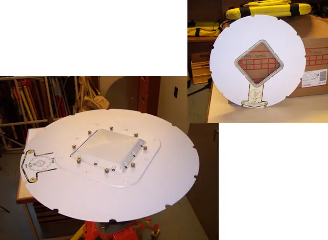
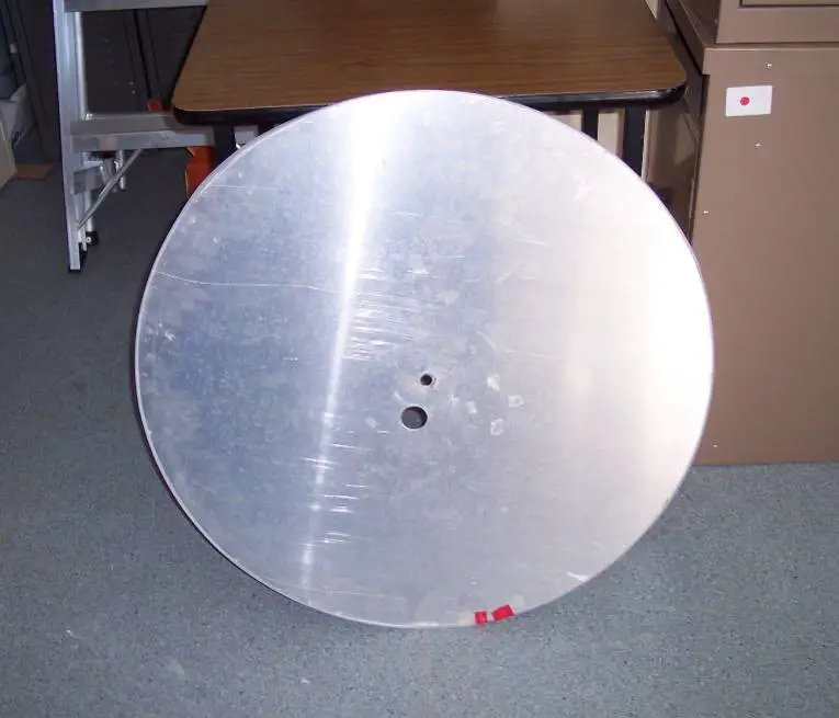
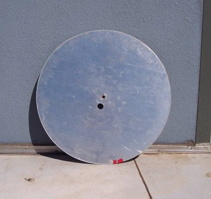
To simulate the effect of multipath during the tests, an 800 millimetre diameter aluminium disc was secured beneath the antenna during the testing. This ‘multipath plane’ is pictured in Figure 2.4.2.
“It is expected that the piece of aluminium will reflect signals so they arrive at the antenna by an indirect route” (McCabe 2002, p. 31) because the multipath plane will be fixed beneath the antenna, thus bouncing multipath into the antenna. Aluminium was used as it was identified in the literature review that foil faced insulation had the greatest effect on antennas, which aluminium has similar properties to (McCabe 2002, p. 16). McCabe decided this method of antenna testing would be the most appropriate compared to methods which used multipath simulation software, as this was testing the effect of multipath on the GPS antenna, not the GPS receiver like the software would do (McCabe 2002, p. 30). 24 hours was also adopted as the minimum observation period as Trimble Navigation has adopted a 24 hour observation period as an acceptable period to log data for and to make comparisons to different days (McCabe 2002, p. 20). The reason for this is that it takes a GPS satellite approximately 12 hours to complete one full orbit of the earth, a 24 hour observation period would allow each satellite to be viewed twice. Comparisons would then be able to be made between different data sets with the analyst being confident that observations on other days would experience similar satellite geometry.
RTK Collector was used to automate the initialisation and loss of initialisation process of the receiver as it was in Manuel’s (2000) testing. As the antenna was in a clear environment 90 seconds was chosen as the optimal time for RTK testing with 30 seconds being the resetting time. 30 seconds was chosen as the resetting time so that the last set of resolved integer ambiguities were not retained (McCabe 2002, p. 34).
McCabe (2002) discovered that the multipath plane did not have a significant impact on the mean TTFF between the test antennas, or the accuracy and precision of any of the test antennas. It is suspected that the minimal difference between the horizontal and vertical coordinate accuracy of each receiver under the two scenarios (with and without the multipath plane) was due to the multipath suppression software ‘Everest’. This software appeared to operate correctly with no major errors in the horizontal or vertical accuracy (McCabe 2002, p. 85).
The effect of multipath was most noticeable when comparisons were made between the percentages of observations outside the manufacture’s specifications before and after the multipath plane was fixed beneath the antenna. Observations which were greater than one standard deviation away from the true coordinates were considered outliers.
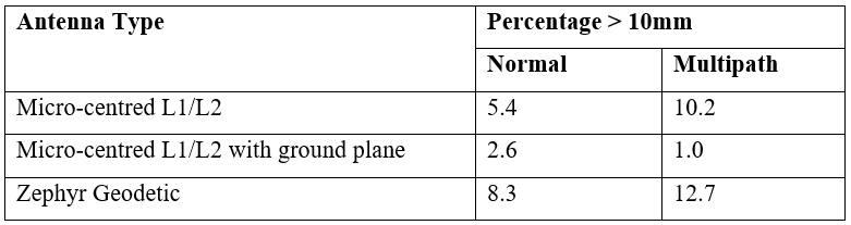
Similar results were also produced in regards to the percentage of vertical observations outside of the manufacturer’s specifications.
The multipath did not impact on the accuracy or precision of the test receivers without any multipath mitigation equipment (i.e. ground plane), but the reliability of the receiver was greatly reduced. This is shown in Table 2.4.1 by the increased percentage of observations which are outside the manufacturer’s specifications.
2.4.4 Research undertaken by Lau (2005)
Previously research completed on multiple-frequency GNSS data processing has tended to concentrate on the availability of more frequencies to solve signal ambiguities. Lau’s primary interest in his research focused on the ability of a multiple-frequency GNSS to resolve signal ambiguities whilst multipath is present. Lau only used the frequencies that would be available from GPS and Galileo satellites. The GLONASS constellation was omitted from the research as at the time of Lau’s research the status of the development/replenishment was unknown (Lau 2005, p. 28).
A GNSS data simulator was developed to generate multipath contaminated data. As expected, the positioning accuracy and precision substantially improved when more signals were available in a clear environment when multipath was not present. However when a reflector was present within about one metre of the antenna, Lau found that positioning results of the GNSS receiver had degraded further than when compared to the GPS receiver. If the receiver-antenna distance is greater than one metre, the multiple-frequency system will have significantly better multipath mitigation capabilities (Lau 2005, p. 202).
Lau (2005, p. 202) concluded that the degraded results were because of the additional measurements from closely allocated frequencies, and when the antenna-reflector distance is less than one metre, the phase multipath errors from GPS and Galileo are highly correlated. A very close reflector will destroy the advantages of using a multiple-frequency GNSS data (Lau 2005, p. 258), advantages which include increased precision, accuracy and TTFF.
2.5 Summary
This chapter introduced the potential benefits that a GNSS capable receiver is able to offer users. Through reviewing the current literature it is evident that there has been no research testing the compatibility of the two navigation systems GPS and GLONASS when in the presence of high multipath. It is important that professionals who rely on this technology be aware of the combined performance of these two GNSSs.
Multipath is a dominant source of error in RTK applications and can impact on the accuracy, precision and the time to first fix of the receivers. It has been found in previous literature that combined usage of signals from multiple GNSSs can potentially degrade positioning results. Practical testing will be required to identify whether combined usage of GPS and GLONASS will either degrade or enhance the chances of a successful initialisation, the TTFF, accuracy and precision of RTK GNSS receivers.
To test the compatibility of the combined use of GPS and GLONASS satellite navigation systems, multipath resistance tests will be completed using the surveying technique RTK GNSS. The results of this test will be compared to RTK GPS to determine if receiver performance has either increased or decreased. Chapter 3 will cover the test methodology and data processing methods for this project.
Chapter 3 – Test Methodology and Data Processing
3.1. Introduction
Chapter two provided background information in relation to the potential compatibility issues between different GNSS constellations and described previous testing procedures. It also demonstrated that there is a current lack of practical research of GNSS and its operation in a high multipath environment. So comparisons may be able to be made between this research and pervious research similar testing procedures and data reduction methods will be adopted.
Chapter 3 will detail all aspects of the testing method to the procedures that will be adopted to analyse the raw information. This ensures that the reproduction of this project is possible.
To properly assess the initialisation integrity of GPS compared to GPS and GLONASS combined there are several factors to be considered: the test location; test regime; field execution and data processing method. Once the raw observations have been processed, it will then be necessary to analyse the observations. Statistics from the observations will be calculated from the processed observation data in Microsoft Excel. The process of how this is done will be explained in the following chapter.
3.2. Test location and Facilities
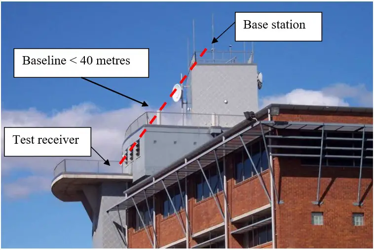
3.2.1. Semi-Permanent GNSS Base Station
Installed on the roof (level 7) of the University of Southern Queensland’s Engineering and Surveying building (Z-block) is a semi-permanent GNSS base station. The base station antenna is a Zephyr Geodetic Model 2 Antenna.
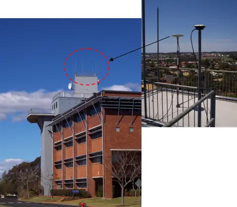
“The base station is painted red and white and is plumbed over a Permanent Survey Mark (PSM) with Map Grid of Australia (MGA) coordinates. Lightning protection devices are installed to protect the GNSS antenna, each one is augmented with independent fuses in all cables that come from the roof” (McCabe 2002, p. 25).
The remaining base station equipment is housed in the computer hut on level 5 of Z-block. This includes the Trimble NetR5 receiver which is capable of observing information from multiple GNSSs, and the computers which control the base station.
3.2.2. Test Location
The location to complete the testing ideally had to satisfy several criteria for it to be suitable:
- Access to mains power to provide a reliable power source for both the antenna and laptop;
- An area to keep the laptop secure and protect it from the weather;
- Able to simulate difficult conditions that are faced by surveyors in each working day (i.e. obstructed satellite window and multipath present);
- Able to set up the equipment and be free from human interference; and
- Have easy access to the equipment and laptop to be able to periodically monitor testing to ensure it was still operating correctly.
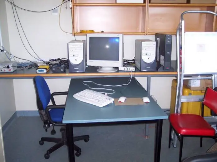
The test location that satisfies all of these criteria is situated on level 5 of the Z-Block roof. Here the laptop is able to be housed in the same computer hut as the base station receiver. The laptop was connected to the receiver through a services duct. Both the laptop and receiver have access to mains power within the computer hut.
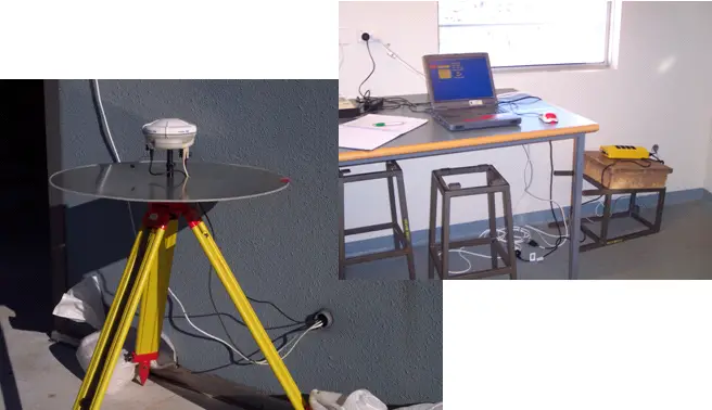
The receiver was established next to the wall which will obstruct almost half of the antenna satellite window. The antenna is situated next to a concrete wall so it is expected that multipath will be present. The reason for establishing the antenna in such a difficult operating environment is to create a commonly faced scenario that spatial professionals work in frequently. It is not uncommon for the user to be working next to tall building or in an open pit mine where both the satellite window will be blocked, as well as having a high presence of multipath, and as stated in Chapter 1 the aim of this research is to test the receiver under conditions which are other than ideal.
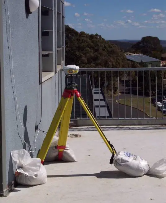
As the antenna does not have a line-of-sight vision to the base station radio this will most likely cause the communication between the base station and rover receiver to be unreliable (Lemmon & Gerdan 1999, p. 65). To over come this, a repeater radio will be setup on level 6 of Z-block to propagate the base station signal ensuring that a robust signal is maintained at all times.

It was decided that testing should only be conducted at the test site already described, and no further testing should be conducted at a test site where the satellite window isn’t obstructed, and where multipath would be negligible. The reason for this is that it has already been proven that “all the interoperability issues that might affect combined use of GPS and GLONASS have been resolved” (Zinoviev 2005, p. 1056), thus it is seen as unnecessary to complete testing in an operating environment where there will be no obstructions.
3.3 Equipment
The equipment required to complete the testing of this project is as follows:
- Laptop (with RTK Collector and Trimble Configuration Toolbox installed);
- Tape measure (to conduct checks of the antenna height);
- Db9 serial connection leads (to connect the antenna to the laptop);
- Trimble docking station (external power supply for SPS880 antenna);
- Tripod;
- Multipath plane;
- SPS880 receiver;
- Adaptor to connect SPS880 to tribrach;
- Tribrach.
The equipment requirements for the required repeater are as follows.
- Repeater;
- Pillar cap;
- Repeater adaptor (to plug repeater into mains power).
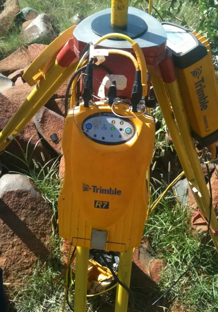
3.4 The Trimble SPS880 Antenna
The antenna to be tested is the Trimble SPS880 GPS antenna. This antenna has an integrated radio, GNSS receiver, GNSS antenna and internal battery. Bluetooth technology allows a cord-less connection between the receiver and surveyor controller. The firmware version that was installed in the receiver during testing was v3.25.
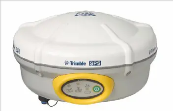
The receiver has 72-channels and tracks L1, L2, L2C, L5 and GLONASS satellites. This availability of a greater number of satellite frequencies from GLONASS is expected to increase satellite coverage and increase the areas where GNSS receivers are able to be operated (Trimble SPS880 Extreme Smart GPS Antenna 2006).
When used with RTK positioning Trimble states that this receiver will provide a horizontal accuracy of ±(10mm + 1 parts per million (ppm) × baseline length) and a vertical accuracy of ±(20mm + 1ppm × baseline length) (Trimble SPS880 Extreme Smart GPS Antenna 2006). The baseline length for testing is less than 40 metres so this means the parts per million for this length will equal less than one millimetre (40m × 10-6 = 4 × 10⁻⁵) and thus will be negligible.
3.5 Test Design
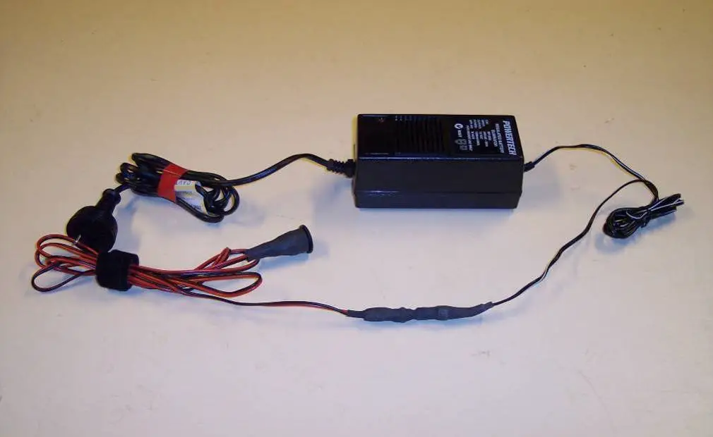
The importance of completing each test over a 24 hour period had been identified in the literature review (section 2.4.3). To do this the laptop, antenna and repeater have to be connected to a mains power supply as portable battery power will not last a sufficient amount of time. This most important criterion was satisfied with the chosen test location.
The laptop came with an external charging device and a Trimble docking station will be used to power the SPS880 antenna. The repeater however will require a power pack to be assembled so it will be able to be powered from a mains power outlet. This was completed by a USQ Electronics Technical Officer.
The other important aspects of this project were: having the laptop communicate with the receiver; and automating the receiver initialisation process. This required two different software programs: Trimble Configuration Toolbox; and RTK Collector Software, both of which will be discussed in further detail in the following two sections.
There are four tests to be completed during this project:
- Observing solely GPS for 24 hours;
- Observing GPS and GLONASS for 24 hours;
- Observing solely GPS with multipath plane fixed beneath it (to enhance the multipath effect) for 24 hours; and
- Observing GPS and GLONASS with multipath plane fixed beneath it for 24 hours.
The multipath plane to be used in the testing is the same one that was used in McCabe’s (2002) research project, which has already been proven to degrade the receiver performance when it is present (section 2.4.3).
Each 24 hour observation period was divided into three eight hour periods. This was due to an unknown fault in the RTK Collector software, after approximately ten hours had passed in the 24 hour observation period the receiver’s baud rate would be reset to the factory defaults. This then meant that information could not be sent from the receiver via the serial connection to the laptop as they were unable to communicate. Resetting the receiver each eight hours did not affect the integrity of the observation data as resetting time only took approximately three minutes each time. As this only occurred twice throughout the 24 hour observation period, the impact on the final statistics was minimal.
An analysis of each of these four tests would be able to provide several different conclusions as to the combined performance of GPS and GLONASS both with and without the multipath plane, compared to the performance of GPS both with and without the multipath plane. It will determine if; there is an increased chance of initialisation when using both satellite constellations, if there is an improvement in accuracy and precision, if there will be an increase in the percentage of successful initialisations and if there is an increased TTFF.
3.5.1 Trimble Configuration Toolbox
The Trimble Configuration Toolbox is a free program available from Trimble’s website. It was used to create a configuration file which allows the user to determine the:
- File name of the configuration file;
- General settings (PDOP, satellite elevation mask);
- The communication parameters between the receiver and laptop;
- The latitude and longitude of the reference station;
- The satellite configuration of the receiver (GLONASS and/or GPS);
- The output NMEA-0183 file;
- Height of the antenna; and the
- Coordinate system.
In previous projects the Trimble Survey Controller (TSC) was used to create the configuration files, however with the latest release of the survey controller TSC2 it is not possible to edit some of the settings which are required to enable the laptop to communicate with the receiver, and to edit the output NMEA-0183 message string.
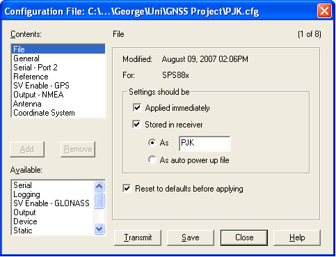
All of these options in the contents section in Figure 3.5.2 were necessary to ensure that observation data was being transferred to the laptop correctly.
3.5.2 Data Logging
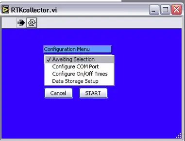
Another important aspect of the testing of this project was to be able to control the receiver over each of the 24 hour testing period without any human intervention. This was done by using a program called RTK Collector. RTK Collector was developed by a USQ Research Technologists using LabView. It was initially developed for Manuel’s (2000) testing (section 2.4.2), however has since been used in one other research project which was by McCabe (2002) (section 2.4.3).
RTK Collector has three sub menus (Figure 3.5.2) which allows the user to determine several parameters of the testing. The three sub menus which are present are; Configure COM Port, Configure On/Off Times and Data Storage Setup. The Configure COM Port menu allows the user to determine the communication parameters at which the laptop is to communicate with the receiver. The Configure On/Off Times menu allows the user to determine the time that the receiver is switched on and switched off for. The Data Storage Setup allows the user to determine where the RTK observation will be saved.
As the antenna was setup in an intentionally obtrusive environment with almost 50% of the satellite window being obstructed, the observation time will be 180 seconds. This will ensure that there is ample time for the receiver to gain a fixed solution provided that there are enough satellites available. The resetting time of the receiver will be 30 seconds. This was identified by McCabe (2002) so the receiver did not retain the last set of resolved ambiguities, and thereby cause a bias in the statistical results.
3.6 Creation of Multipath Environment
To generate a high level of multipath during the tests the same method used by McCabe (2002) will be adopted. McCabe secured an 800mm diameter aluminium disc beneath his GPS test antennas. It was identified in his conclusion that the presence of this multipath plane did affect the receivers performance (McCabe 2002, p. 84). Some results of his testing are repeated in section 2.4.3.
It is expected that multipath will already be present during the testing without the multipath plane. This will be due to the concrete wall and concrete surface, however with the multipath plane present it is expected that a much higher level of multipath will be generated.
3.7 Data Processing
The processing of the observation data was an important part of this project. It was important to where possible to adopt the methods of filtering the observation data to ensure comparability of the results from this research project to the results of other projects. The following sections will detail and justify the methods of processing and reducing the observation data files.
3.7.1 NMEA-0183 Output Message
The NMEA-0183 output message was an option in the Trimble Configuration Toolbox when creating a configuration file. The NMEA output message adopted for this project was PTNL, PJK. An example of a PTNL, PJK NMEA output file is shown in Appendix B.
3.7.2 Reduction of Observation Data
Before information and statistics could be drawn from the observation data, it first had to be reduced to only what will be required in the analysis. Reducing the observation data included; removing all the information other than the time when the receiver turned on and then became initialised, determining the UTC (Universal Time Coordinated) for when the receiver first switched on from the first line of the initialisation (as until the observation has a fixed solution, the receiver cannot determine the correct UTC), doing this meant that the time taken for the receiver to initialise could now be calculated. Also removing the observation periods where an initialisation did not occur.
What remained after the reduction were two lines of each successful initialisation; the line when the receiver turned on, and the first line when the receiver initialised, an example of which is shown in Appendix E. All of this was done manually in Microsoft Excel.
3.7.3 True Coordinates
The purpose of completing all tests over a single point was so that the accuracy and precision of the horizontal and vertical coordinates of each test could be compared to one another. So they can be compared first the ‘true coordinates’ of the test point (screw in concrete) need to be calculated to provide a relative point of comparison.
The ‘true coordinates’ were calculated using the GPS observation data. It was decided that the GPS observation data will have any observation outside 1.96 times (95% confidence interval) the manufacturer’s specification for baseline component standard deviation from the reiterative mean to be removed. A 95% confidence interval was chosen as it was desired that the ‘true coordinates’ have a stricter filter than what will be used to produce the statistics, which will be further explained in the following section.
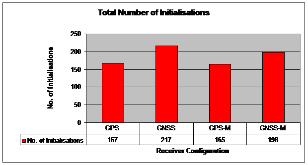
3.7.4 Total Number of Initialisations
Once all that was remaining in each observation file was the line when the receiver initially turned on and when the receiver first initialised, to calculate the total number of successful initialisations was a simple process. All that was required was to count the entire number of lines in the observation data file, and then divide this value by two.
3.7.5 Time to First Fix (TTFF)
The NMEA-0183 time values are presented in UTC and are represented as hhmmss, where:
- hh is hours, from 00 through 23;
- mm is minutes; and
- ss is seconds.
For ease of calculation the TTFF values were converted into seconds. To do this the single cell containing the UTC was split up, then each of the hh and mm cells were converted to seconds and then both summed to the ss cell. Then to calculate the TTFF, the seconds from the receiver switching on line were subtracted from seconds of the initialisation line.
3.7.6 Horizontal Coordinate Accuracy and Precision
To determine the precision and accuracy of the horizontal coordinates first the difference between the ‘true coordinates’ and the observation coordinates had to be found. These calculations were completed in Microsoft Excel by assigning formulas to cells. The difference in the easting and northing now had to be converted to a distance value, this was done using Pythagoras theorem: Horizontal Distance = SQRT (ΔE2 + ΔN2). Once the horizontal distance away from the true coordinates had been calculated a statistical analysis on these observations was carried out.
As it is expected that there will be a large number of gross observations, two charts will be produced; one showing the accuracy and precision of all initialisations, the second chart showing the accuracy and precision of the filtered observations. To determine if an observation is an outlier the same test will be adopted that Lemmon & Gerdan (1999) adopted for their testing, and that is to consider an observation to be an outlier if it is more than three times the manufacturer’s specifications for the baseline component standard deviation. This second chart will allow comments about the accuracy and precision of the receiver configurations and operating environments to be made.
3.7.7 Ellipsoidal Height Accuracy and Precision
To determine the precision and accuracy of the ellipsoidal heights first the difference between the ‘true’ ellipsoidal height and the observation ellipsoidal height had to be found. This calculation was completed using Microsoft Excel. Once the differences had been calculated statistics such as the mean and standard deviation could be calculated.
Just as detailed in section 3.7.6 two ellipsoidal height accuracy and precision charts will be produced; one chart showing the accuracy and precision of all successful initialisations, the second chart showing the accuracy and precision of the filtered observations. The same filtering technique as described in section 3.7.6 will be used, which is to filter ellipsoidal height observations which are greater than three times the manufacturer’s specifications for the baseline component standard deviation.
3.7.8 Outlying Observations
As identified in section 2.4.3, McCabe (2002) found the main differing in the performance of the receivers with the multipath plane and the receivers without the multipath plane was the percentage of outlying initialisations which occurred. It is for this reason that it is seen as important the number of outlying observations form a part of the analysis. As specified in the two previous sections an outlying observation will once again be considered to be an observation which is greater than three standard deviations from the true coordinates.
3.8 Summary
This chapter outlined the required equipment for this testing, the tests that will be completed, the software that will be used to complete the tests and the method to reduce and process the observation data. The test location that was chosen to complete all four tests was also justified.
Each testing period will last for 24 hours, with the receiver logging information for 180 seconds and then resetting for 30 seconds. Microsoft Excel will be the program used to complete a statistical analysis on the data allowing for some conclusions to be drawn from it about the performance of GPS and GLONASS combined.
The next chapter will present the results of the statistical analysis taken place. It is expected conclusions about the performance of GPS and GLONASS will be able to be drawn from this chapter.
Chapter 4 – Results
4.1. Introduction
Chapter 3 discussed the testing methodology and data processing method that will be used in this project. It also justified these testing procedures, as well as the location of testing and the use of the multipath plane.
Chapter 4 will present each of the charts that will be used throughout the analysis. The full detailed analysis of these results will be covered in Chapter 5.
This chapter comprises of two sections, the processing of the raw data and the collation and analyse technique used to analyse the data. Microsoft Excel was used to both process the raw data and to collate and compare all the results.
4.2. Results
4.2.1. True Coordinates
It is with the process detailed in section 3.7.3 the following ‘true coordinates’ coordinates were calculated:
| Easting | Northing | Ellipsoidal Height | |
| ‘True coordinates’ of test location | 394480.108 m | 6946310.805 m | 725.834 m |
4.2.2. Total Number of Initialisations
The total number of observations for each of the test periods is shown in Figure 4.2.1.
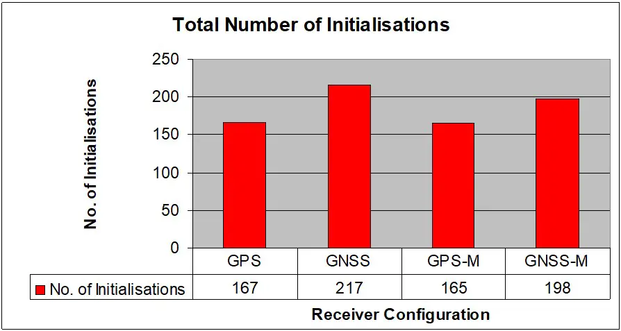
The GPS and GNSS tests were in a low multipath environment (multipath generated from concrete wall), while the M at the end of GPS-M and GNSS-M signifies that the multipath plane was present. Figure 4.2.1 will be further discussed in Chapter 5.
4.2.3. Time to First Fix
Figure 4.2.2 shows the mean and standard deviation of the TTFF for each test, the high and low bar represent one standard deviation either side of the mean.
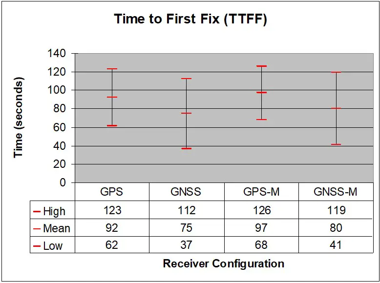
Table 4.2.2 shows another composition of the TTFF.
| GPS | GNSS | GPS-M | GNSS-M | |
| % < 60 seconds | 11 | 49 | 8 | 43 |
| 60 < % < 90 seconds | 41 | 21 | 39 | 24 |
| % > 90 seconds | 48 | 29 | 53 | 33 |
4.2.4. Horizontal Coordinate Precision and Accuracy
Initially the mean and standard deviation of each successful initialisation was calculated and graphed in Figure 4.2.3.
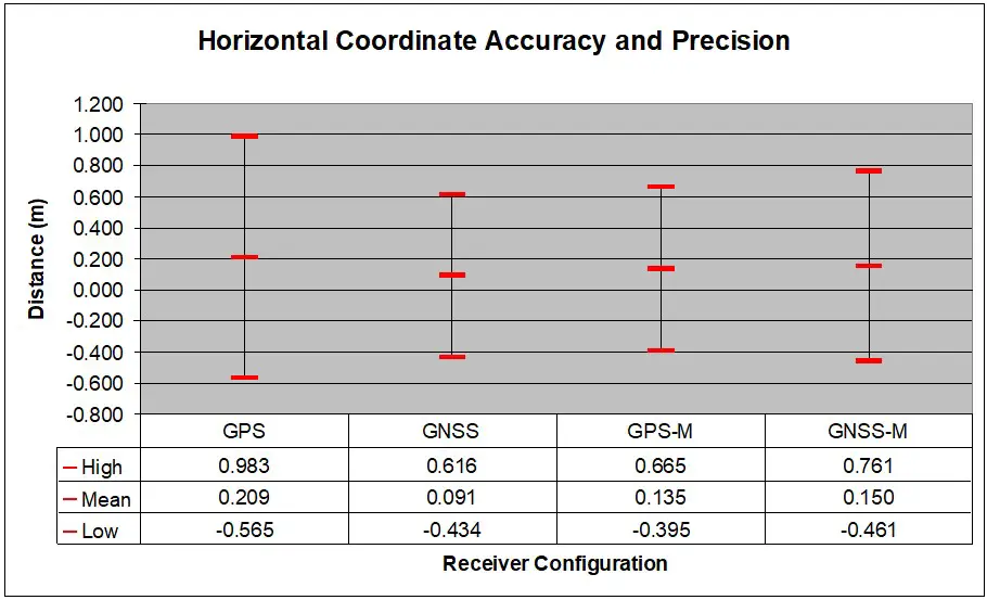
The high and low bar represent one standard deviation either side of the mean of the horizontal distances.
It is obvious that there are numerous outlying observations which are impacting the mean and standard deviation of the horizontal coordinates. For this reason it is necessary to produce a horizontal coordinate accuracy and precision chart which has had all outlying observations filtered (for method see section 3.7.6). Trimble had specified for the test antenna the SPS880, the expected horizontal accuracy is ±(10mm + 1ppm) (Trimble SPS880 Extreme Smart GPS Antenna 2006, p. 3). The filtering limits for the horizontal coordinate will be set at: 3 × ±(10mm + 40m × 10-6) = ±0.030m. This resulted in Figure 4.2.4.
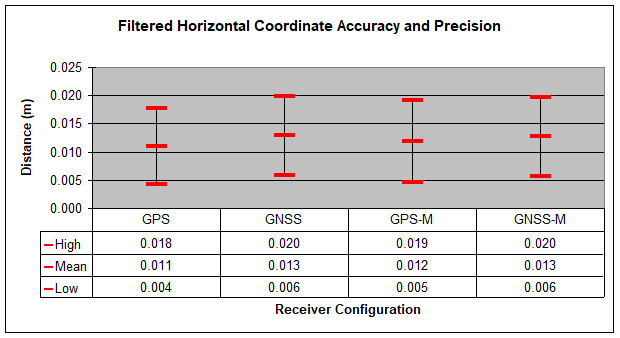
This chart will not form part of the analysis in Chapter 5, instead was just shown here to demonstrate that when outlying observations are removed, the accuracy and precision of both receiver configurations with and without the multipath plane are comparable. It will not be used in the final analysis as all it proves that once all the ‘bad’ initialisations are removed, what is left is ‘good’ statistics (which appear free from error). Figure 4.2.3 will be reproduced in section 5.2.3 and will be discussed as while it is adversely impacted upon by large outlying initialisations, it does contain more information of what is happening.
4.2.5. Vertical Coordinate Accuracy and Precision
The mean and standard deviation of each successful initialisation of each test is shown in Figure 4.2.5.
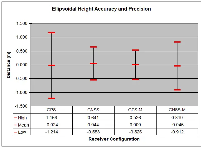
As with the horizontal coordinate accuracy and precision chart (Figure 4.2.3) the standard deviations are obviously being influenced by large outlying observations. In this case the specified ellipsoidal height accuracy is ±(20mm + 1ppm) (Trimble SPS880 Extreme Smart GPS Antenna 2006, p. 3). The filtering limit for the ellipsoidal height will be: 3 × ±(20mm + 40m × 10-6) = ±0.060m. Once the outlying observations had been filtered the following graph was produced.
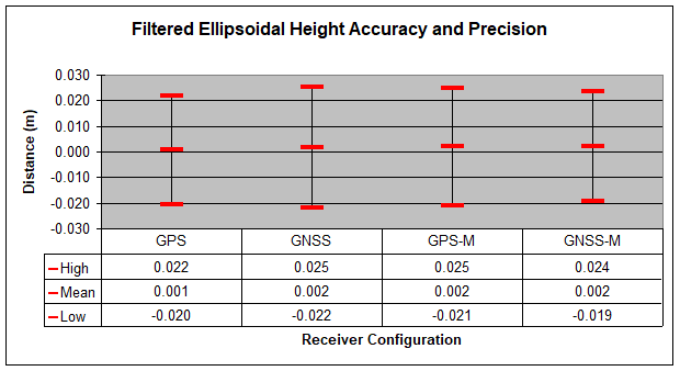
Figure 4.2.6 shows that once the outlying observations are removed the accuracy and precision of each of the tests are comparable. As stated in section 4.2.3, all Figure 4.2.6 proves is that once the ‘bad’ observations are removed, ‘good’ statistics are produced. This figure will not be used in the analysis in Chapter 5 as it does not show what is really occurring. This chart however does show that without the outlying observations the accuracy and precision of both receiver configurations with and without the multipath plane are comparable.
4.2.6. Outlying Observations
Figure 4.2.7 shows the percentage of horizontal coordinate observations which fall outside three sigma from the true coordinates.
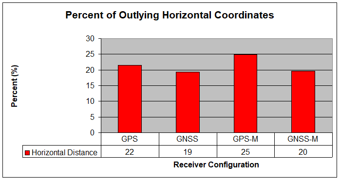
Figure 4.2.8 shows the percentage of outlying ellipsoidal height observations from the true coordinates. The filter is the same as specified in section 4.2.6.
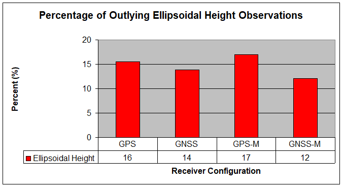
These two charts both show similar trends, but the chart that will be used in Chapter 5 to form part of the analysis will be Figure 4.2.9. This chart shows the percentage of total observations which have either one or both measurement elements (horizontal coordinate or ellipsoidal height) outside three sigma from the true coordinates. Figure 4.2.9 was chosen over using both Figure 4.2.7 and Figure 4.2.8 because it avoids unnecessary duplication of the figures.
4.3. Summary
The Charts presented in Chapter 4 will form an important part of the final analysis of the performance of the two receiver configurations in both a low and high multipath environment.
It was explained that the filtered accuracy and precision charts will not be used in the final analysis of the observations. The reason for this is so the real picture of what is occurring is shown, not one which looks good and is easier to explain. From preliminary observations it can be seen that there are some anomalies affecting the accuracy and precision charts, what is occurring here will have to be investigated and explained.
Chapter 5 will discuss relevant charts presented in Chapter 4 and will have a complete analysis of the performance difference between the two receiver configurations in both a low and high multipath environment.
CHAPTER 5 – RESULTS ANALYSIS AND IMPLICATIONS
5.1. Introduction
The results from the analysis of the raw data have been detailed in Chapter 4. It is now necessary to address the aim of this project and to combine the different data sets allowing conclusions to be made about the performance of combined GPS and GLONASS data compared to the performance of solely GPS data.
This Chapter will present the combined results presented in Chapter 4 of each of the four tests completed. A comparison between the results will then address the aim of this research project detailing the differences in; precision, accuracy and TTFF.
This chapter comprises of two main sections: the results analysis section and the implications section. As stated in the aim an analysis of the accuracy, precision, TTFF and the number of successful initialisations for each receiver configuration will be compared. Then the second section will discuss the implications of these results on the professionals who rely on this technology daily.
5.2. Results Analysis
5.2.1. Number of Initialisations
The total number of initialisations is an important measure in showing what benefits will result as a greater number of satellites become available for the users receiver. As expected, GNSS outperformed GPS, both with and without the multipath plane. This was due to the wider satellite coverage with additional GLONASS satellites. This is shown in Figure 5.2.1.
Whilst there are a greater number of observations made over the 24 hour period from GNSS, this does not mean that GNSS was the better performer. This information will be used in conjunction with the vertical and horizontal coordinate information so conclusions on the performance of both receiver configurations can be made.
5.2.2. Time to First Fix (TTFF)
The TTFF is an important measure of an RTK receiver efficiency. Obviously the longer the time taken to initialise the less productive the receiver is. Figure 5.2.2 combines the TTFF for each of the receiver configurations to allow for ease of analysis.
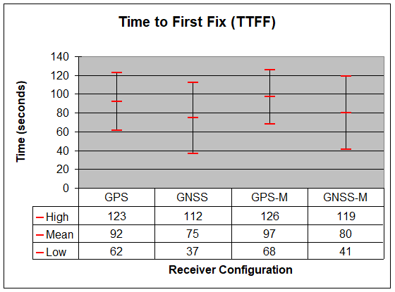
This figure shows the mean TTFF of all successful initialisations. The high and low bar represent one standard deviation either side of the mean to show the spread of the data.
Figure 5.2.2 shows that there is a clear increase in performance of the GNSS receiver configuration over the GPS receiver configuration both with and without the multipath plane. The multipath plane also did have a clear impact on the time taken for the receiver to initialise between the same receiver configurations. Figure 5.2.2 clearly shows that the presence of additional satellites improved the receivers TTFF. In both cases of GNSS v GPS with and without the multipath plane the average TTFF was decreased by 17 seconds. This is quite a substantial improvement and will equal improved efficiency in the field. The difference between the same receiver configurations was less noticeable with 5 seconds being the difference in both cases.
One notable difference between the GPS and GNSS receiver configuration is that the standard deviation of the GNSS receiver is larger that the standard deviation of the GPS receiver. This shows that there is a greater spread of the TTFF for GNSS. However the range of the GNSS standard deviation falls within the peak of the GPS still signalling that the performance is improved overall.
5.2.3. Horizontal Coordinate Accuracy and Precision
The accuracy and precision of the horizontal coordinates not only appears to contradict Figure 5.2.2, but it also appears to contradict itself. As shown in Figure 5.2.3 when comparing the horizontal coordinate accuracy and precision of GPS v GNSS against the results of GPS-M v GNSS-M the results show almost a mirror effect in performance.
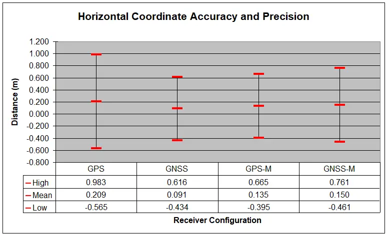
The mean bar represents the average distance from the true coordinates of all successful initialisations. The high and low bars are one standard deviation either side of the mean.
The GNSS receiver significantly outperformed the GPS receiver with the average distance away from the mean improving by 0.118m. Also its measurements have a greater level of repeatability when compared to GPS. This is shown by the reduced magnitude of the standard deviation. Under normal conditions so far it can be seen that GNSS significantly out performs GPS however, the contradiction as already alluded to comes when viewing the GPS-M data and GNSS-M data. The average distance of the GPS-M data is closer to the true coordinates and has the smaller standard deviation than GNSS-M. This is the opposite of what happened to the data when there is no multipath plane.
The most interesting point to make of this data is that the GPS-M outperformed GPS in both accuracy and precision. This is definitely not what was expected of the results as the multipath plane has already been proved to decrease receiver performance as previously specified in section 2.4.3. The ellipsoidal height accuracy and precision will now be analysed to see if a similar trend has occurred, then the reasons for the apparent contradiction in the horizontal coordinates will be discussed.
5.2.4. Ellipsoidal Height Accuracy and Precision
Figure 5.2.4 looks very similar to the results that were produced in Figure 5.2.3, with the apparent contradiction between the results without the multipath plane compared to the results with a multipath plane.

The mean bar represents the mean of all ellipsoidal height observations while the high and low bar represent one standard deviation either side of the mean.
A difference between the ellipsoidal height and horizontal coordinate accuracy and precision charts is that GPS outperformed the accuracy of GNSS, however the range of a single standard deviation either side of the mean of the GNSS observations falls well within the magnitude of the GPS data. This shows how much more precise the results are when there are additional satellites available.
Apart from that one difference the results shown in Figure 5.2.4 are very similar to what has already been discussed in section 5.2.3, including the out performance of GPS-M over GPS.
It is clear that there is some anomaly impacting on the mean and standard deviation of Figure 5.2.3 and Figure 5.2.4, further information will need to be extracted from the observation data to determine what is occurring, and if there is a possible compatibility issue between the GPS and GLONASS satellite constellations.
5.2.5. Outlying Observations
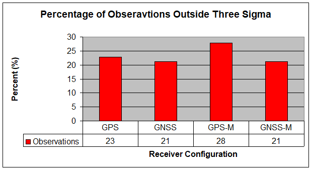
The observation data which is being used to generate the statistics currently seen in Figure 5.2.3 and Figure 5.2.4 is such far is unfiltered. As shown in Chapter 4 the reason that the horizontal distance and ellipsoidal height statistics look so poor is that there are large outlying observations within the observation data. To determine if it is these outlying observations which are giving a false impression of the actual performance of the receiver, the outlying observations will be shown as a percentage of the total number of initialisations for the respective receiver configuration. Figure 5.2.5 shows the percentage of total initialisations which fall outside three sigma (99.74% confidence interval) of the true coordinates.
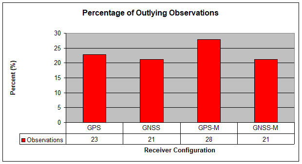
Figure 5.2.5 already shows important information even without comparing it to other information. Firstly multipath clearly adversely impacted on the GPS receiver configuration with the number of outlying observations increasing by 5% with the multipath plane. Another important piece of information is the equal performance of the GNSS receiver both with and without the multipath plane. This does suggest that with the additional GLONASS satellites the receiver is able to provide a more robust initialisation and can filter out bad signals more effectively. These results suggest that the satellite constellations GPS and GLONASS are compatible when used simultaneously with each other.
Figure 5.2.5 does contradict Figure 5.2.3 and Figure 5.2.4 as GPS-M outperforms both GNSS-M and GPS in terms of precision and accuracy however, it can be seen clearly in Figure 5.2.5 that it also has the greater number of outlying observations. This additional information shows that the initialisation reliability of GPS-M is less than both GNSS-M and GPS. The most likely reason that this greater percentage of outlying observations is not reflected in the mean and standard deviation of GPS-M in Figure 5.2.3 and Figure 5.2.4 is that GPS and GNSS-M outlying observations have, for some reason a greater magnitude than the outlying observations of GPS-M.
Due to the poor standard deviation of both GNSS-M and GPS, it can be assumed that the reason the statistics look so poor is that the outlying observations have for some reason a larger magnitude from the mean. This can be confirmed by viewing the maximum and minimum of each test and comparing them.
5.2.6. Observation Range
Figure 5.2.6 and Figure 5.2.7 show the observation range of the ellipsoidal height and horizontal distance respectively.
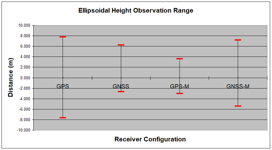
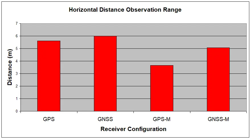
Figure 5.2.6 and Figure 5.2.7 show what was expected and that is that GPS-M outliers had a reduced magnitude compared to GNSS-M and GPS. These two figures show only one observation which is furthest away form the mean, however they both provide a good explanation as to why the standard deviation of both GNSS-M and GPS were so large.
5.3. Implications of Research
From the information above it is clear that the GNSS receiver outperforms the GPS receiver in terms of all elements related to the performance of a receiver as stated in Chapter 1. The following points support this claim:
- The GNSS receiver recorded a greater number of observations compared to the GPS receiver. This is because of the wider coverage of satellites available when observing both GPS and GLONASS. This shows the benefits that a GNSS receiver would offer to a user where work must be completed in areas where the satellite window is obstructed.
- The average TTFF of the GNSS receiver both with and without the multipath plane was faster in comparison to the GPS receiver. Clearly with a greater number of satellites available, the receiver was able to initialise much faster.
- The reliability of the GNSS receiver is better than the GPS receiver both with and without the multipath plane. This conclusion has been made in respect to Figure 5.2.5, which shows that the GNSS receiver configuration both with and without the multipath plane has a lesser percentage of observations outside three sigma from the true coordinates.
- The GNSS receiver had better multipath mitigation capabilities than the GPS receiver. This is shown in Figure 5.2.5 with the equal percentage of outlying observations both with and without the multipath plane. Whereas the GPS receiver was clearly impacted upon by the multipath plane, with outlying observations increasing by 5%.
- Figure 5.2.3 and Figure 5.2.4 showed misleading statistics in regards to the accuracy and precision of the horizontal coordinates and ellipsoidal heights of all observations. It was shown in Figure 5.2.5 that there are a large percentage of outlying observations, and Figure 5.2.6 and Figure 5.2.7 showed the range of the largest outlying observation which further confirmed the influence of large outliers on the statistics. Figure 4.2.4 and Figure 4.2.6 showed that once the outliers were removed the accuracy and precision of each test was comparable. These charts were not included in Chapter 5 as this does not show anything other than if all ‘bad’ initialisations are removed, you are left with ‘good’ statistics, and thus were not incorporated into the analysis of the observations.
5.4. Research Gaps
The number of comparisons that are able to be made between each of the four tests is limited as a result of the testing procedures. It was identified in section 2.4.3 that when comparing RTK GPS tests from different days, it is sufficient provided that the observation period has been for 24 hours. As can be seen in the following figure, when the number of satellites used to initialise is shown as a percentage of the total number of initialisations there is quite a substantial difference between both GPS tests.
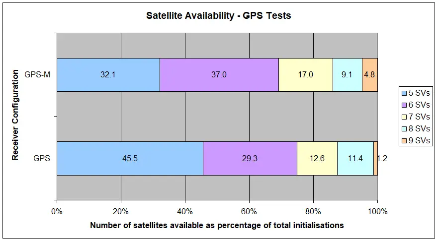
Even though each test was completed over 24 hours and theoretically they are comparable, this chart clearly shows that there are inequitable differences between the two charts with GPS at a clear disadvantage to GPS-M as it had fewer initialisations observing six satellites or more. It is unable to be explained why there is such variation between the two tests in the number of satellites observed.
There was a similar outcome when comparing the two GNSS tests. GLONASS has a 11 hour 15 minute orbiting period (GLONASS – Summary 2001) which will result in an uneven observation period for each of the observations. Also as GLONASS isn’t fully operational yet it is likely that there was also an unbalanced observation periods.
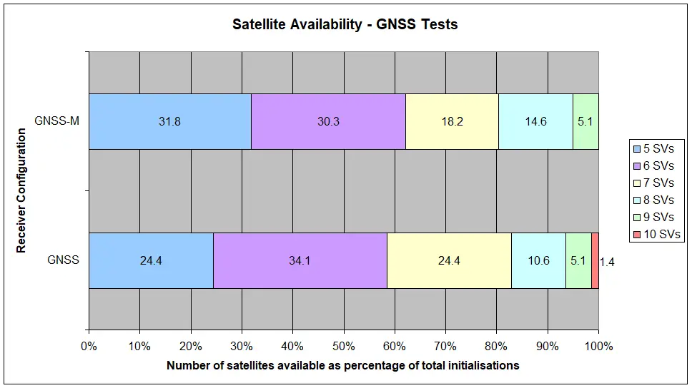
Even though Figure 5.4.1 and Figure 5.4.2 show obvious differences in the number of satellites viewed in each test period between the same receiver configurations, the tests are still able to have comparisons made between them for the purposes of this research project. It did however limit the number of comparisons that could be made between each data set.
Ideally each of these tests would have been completed simultaneously over the same point. This however was not possible due to equipment limitations. A recommendation will be made in Chapter 6 that for future testing of GPS or GNSS receivers that to ensure unbiased comparisons can be made between tests that they be completed simultaneously.
5.5. Other Observations
In Chapter 2, section 2.3.1 it was identified that one reason errors may remain and not be detected in an RTK survey is because of the increasing trend among surveyors to have a shorter occupation time over points. The percentage of observations in a low and high multipath environment with an obstructed satellite window is quite large and further investigation should be completed to determine if occupation time really does improve the accuracy of the RTK position system.
To determine if the observation does correct itself after a period of time, each observation which was greater than three times the manufacturer’s specification for baseline component standard deviation from the true coordinates will be analysed. This then resulted in the following table.
| Total Number of Outlying Observations | Number of Observations which remained in error | Percentage of Observations which remained in error | |
| GPS | 38 | 31 | 81.6 |
| GNSS | 46 | 45 | 97.8 |
| GPS-M | 46 | 36 | 78.3 |
| GNSS-M | 42 | 32 | 76.2 |
| Total | 172 | 144 | 83.7 |
It can be seen clearly in Table 5.5.1 that even if the point is occupied for some time that the receiver does not automatically correct itself and improve its accuracy. This does place a large emphasis on the importance of maintaining the initialisation integrity of the receiver and ensuring that the antenna is in an environment where multipath will be either minimal or nil. It is possible that if the antenna was moving that errors like this would be detected and removed, but unfortunately this cannot be demonstrated with the available information. An example of an observation correcting itself is shown in Appendix C, and an example of an observation not correcting itself is shown in Appendix D.
5.6. Summary
The expected benefits specified in section 2.2.2 that users would expect from additional available satellites have materialised, with all elements of receiver performance as specified in Chapter 1 being improved upon when compared to a receiver observing solely GPS satellites. This included increased number of initialisations, faster TTFF and improved initialisation reliability.
The presence of the multipath plane did have an impact on both receiver configurations by reducing the number of fixed solutions and increasing the TTFF of both receiver configurations, however as shown in Figure 5.2.5 the GNSS receiver showed better multipath mitigation capabilities compared to the GPS receiver by having an equal percentage of outlying observations with and without the multipath plane.
Because of the large percentage of outlying observations, the accuracy and precision charts have been adversely affected by the inconsistent magnitudes of the outlying observations disproportionately impacting upon the mean and standard deviation. This however was over come by using the horizontal distance and ellipsoidal height accuracy and precision charts (Figure 5.2.3 and Figure 5.2.4 respectively) in conjunction with the outlying observations chart (Figure 5.2.5) to provide an accurate analysis of what is occurring.
Chapter six will discuss the final conclusions and recommendations, and outline a future research topic which is related to the further testing of GNSS receivers and multipath resistance testing.
Chapter 6 – Conclusion
6.1. Introduction
The processed and collated results for the number of initialisations, TTFF, accuracy and precision of the GNSS and GPS receiver configuration with and without the multipath plane were processed, analysed and compared in Chapter 4 and Chapter 5.
From this analysis of results, final conclusions can be made as to the performance of a GNSS receiver under a high multipath environment, and whether a GNSS receiver has better multipath mitigation capabilities compared to a GPS receiver.
Chapter 6 will consist of conclusions addressing the aim of the project, followed by recommendations for future research.
6.2. Conclusions
Chapter 1 established the aim of this research project which was to critically analyse the ability of an RTK GNSS receiver to provide more accurate and precise positioning results in a low and high multipath environment compared to an RTK GPS receiver. To achieve the aim each of the elements of receiver performance (number of fixed solutions, TTFF, accuracy and precision) were required to be tested and analysed using the testing procedure outlined in Chapter 3. In the following subsections the conclusions to the elements of receiver performance will be stated.
6.2.1. Number of Initialisations
The GNSS receiver had a greater number of successful initialisations over the 24 hour observation period than the GPS receiver (see Figure 5.2.1). This is a result of the greater satellite coverage with the additional available satellites from the GLONASS constellation. This shows clearly the benefits of a GNSS receiver when working in environments which will obstruct the satellite window.
The multipath plane did have an impact on the number of total initialisations of both receiver configurations with fewer initialisations occurring in its presence. This does show the impact of multipath on the initialisation ability of both GNSS and GPS receivers.
6.2.2. Time to First Fix
The GNSS receiver had a decreased TTFF with 17 seconds being the improvement both with and without the multipath plane compared to the GPS receiver. Although the GNSS receiver TTFF had a greater spread than the GPS receiver indicated by the larger standard deviation, both with and without the multipath plane it was within the peak of the GPS standard deviation. With the greater number of satellites available the receiver is able to solve the signal ambiguities faster thus improving the TTFF. The relationship between the number of satellites in an initialisation and the time taken to initialise has already been investigated by Lemmon & Gerdan (1999) as discussed in section 2.4.1.
The multipath plane did impact on the TTFF of both receiver configurations with 5 seconds being the difference in both cases when comparing the same receiver configurations with and without the multipath plane.
6.2.3. Accuracy and Precision
As discussed in section 5.2.3 and section 5.2.4 the ellipsoidal height and horizontal distance accuracy and precision charts are misleading in the apparent performance they show. The reason for this it was concluded that there were some very large outlying observations which were creating unbalanced statistics. It was shown in Figure 4.2.4 and Figure 4.2.6 that if the outlying observations were removed the accuracy and precision of each of the tests were comparable, as mentioned though this proved nothing more than if bad observations were removed good statistics remained. Using the unfiltered observations in the analysis formed an important part of the analysis as it showed more of what was happening.
To give a better indication of how reliable the results really were the number of initialisations which were three sigma outside the true coordinates were represented as a percentage of the total number of initialisations (Figure 5.2.5). This showed that GNSS had smaller percentage of observations fall three sigma outside the true coordinates, which meant that the GNSS receiver was the more reliable compared to the GPS receiver.
The GNSS receiver also displayed greater multipath mitigation capabilities. This was indicated by the GNSS receiver both with and without the multipath plane having the same percentage of observations outside three sigma from the true coordinates. Whereas the GPS receiver had 5% more observations outside three sigma from the true coordinates, compared to when the multipath plane was not present.
6.3. Additional Comments
It was not part of the original aim of this research project to view, if the receiver was given enough time if it would correct outlying observations at a later point during the initialisation. It was however an interesting observation that 83.7% of the outlying initialisations did not at a later point in the observation correct itself.
This observation shows the importance of maintaining the initialisation integrity of the antenna, ensuring that the initialisation environment has either no multipath or at most minimal levels of multipath.
6.4. Future Research
When a fully operational capability Galileo constellation becomes available, possible future testing could involve the testing and comparing of GPS satellites against Galileo satellites against GPS and Galileo combined. It is recommended all future RTK positioning testing be completed simultaneously as opposed to consecutively, this will ensure that legitimate comparisons can be made between each of the tests. It was shown in Figure 5.4.1 and Figure 5.4.2 that even though the observation period was 24 hours, this did not result in a comparable number of satellites being available over each test period.
This proposed future research is a requirement as RTK positioning technology becomes further integrated with the duties of spatial professionals, there is a requirement that they understand and trust the operation of their equipment under different operating environments (i.e. high multipath) as so more informed decisions are able to be made with respect to what equipment would be more appropriate for a specific task.
6.5. Close
Through testing of the GNSS receiver in both a high and low multipath environment, the multipath mitigation capability of a GNSS receiver has been ascertained. With the additional satellites of GLONASS the GNSS receiver has superior multipath mitigation capabilities than the GPS receiver. This was proven in Chapter 5 which detailed the improvement number of initialisations, TTFF and fewer outlying initialisations (which indicated improved precision and increased reliability).
This research project has enabled a greater level of understanding of the operational characteristics of a GNSS receiver compared to a GPS receiver. For those who are thinking about an investment in a GNSS receiver the advantages of such an investment is clear. This is one technology that will be embraced by spatial professionals, who are continually looking for methods to improve efficiency in the field.
This research project has achieved its aim by critically analysing the ability of a GNSS receiver to perform in a low and high multipath environment compared to a GPS receiver.
List of References
Compass GPS 2007, viewed 30/10/2007, http://www.chinapage.com/.
Defining the Future of Satellite Surveying With Trimble R-Track Technology, 2006, Trimble Engineering and Construction Group, viewed 16/03/2007 http://trl.trimble.com/docushare/dsweb/Get/Document-287233/022543-214_GNSS_WP_0206_Survey.pdf.
El-Rabbany, A 2002, Introduction to GPS – The Global Positioning System, Artech House, Inc., Norwood.
Feng, Y, Rizos, C & Moody, M 2006, ‘Exploring Performance Benefits from Multiple Satellite Systems and Multiple Carrier Signals Using GPS and Virtual Galileo Measurements’, paper presented to International Global Satellite Systems Society, Surfers Paradise.
Geodetic Surveying A – Study Book 2, 2005, University of Southern Queensland, Toowoomba.
Gibbons, G 2006, ‘GNSS Trilogy: Our Story Thus Far’, Inside GNSS, p. 8.
GLONASS – Summary, 2001, Andrews Space & Technology, viewed 22/10/2007 http://www.spaceandtech.com.
GNSS, 2006, Septentrio, viewed 2 April 2007 2007, http://www.septentrio.com/about_gnss.htm.
Higgins, M 2006, ‘Carrier Phased Based Positioning in Australia and in Queensland’, paper presented to US Civil GPS Service Interface Committee Gold Coast.
Higgins, M & Honor, I 1999, Surveying with the Global Positioning System, Department of Natural Resources, QLD.
Lachaleppe, G, Cannon, E, O’Keefe, K & Alves, P 2002, How Will Galileo Improve Positioning Performance?, 16/03/2007, http://www.gpsworld.com/gpsworld/article/articleDetail.jsp?id=30689&pageID=1&sk=&date=.
Lau, L 2005, ‘Phase Multipath Modelling and Mitigation in Multiple Frequency GPS and Galileo Positioning’, PhD thesis, University of London.
Lemmon, TR & Gerdan, GP 1999, ‘The Influence of the Number of Satellites on the Accuracy of RTK GPS Positions’, The Australian Surveyor, vol. 44, no. 1.
Manuel, BJ 2000, ‘Testing the Initialisation Integrity of the Trimble 4700 Real-Time Kinematic Global Positioning System’, University of Southern Queensland.
McCabe, RJ 2002, ‘Performance Testing of the Trimble Zephyr Geodetic GPS Antenna’, University of Southern Queensland.
Thomson, I 2007, China launches GPS rival, Computing, 30/10/2007, http://www.computing.co.uk/.
Trimble 2001, Trimble Virtual reference Station.
Trimble SPS880 Extreme Smart GPS Antenna, 2006, Trimble Construction Division, viewed 17/07/2007 2007.
Trimble SPSx80 Smart GPS Antenna – User Guide, 2006, A edn, Trimble, Sunnyvale.
Wolf, PR & Ghilani, CD 2002, Elementary Surveying – An introduction to Geomatics, 10th Edition edn, Prentice Hall, New Jersey.
Zinoviev, AE 2005, ‘Using GLONASS in Combined GNSS Receivers: Current Status’, paper presented to ION GNSS 18th International Technical Meeting of the Satellite Division, Long Beach.
